The Modal Israeli
Ariel Karlinsky
10/12/2019
Introduction
This markdown contains text and code for the “Modal Israeli” post on The Artist & Merchant, heavily inspired by Planet Money’s episode 936: The Modal American (check it out!)
We will use the Family-Expenditure Survey Micro-data Public Use File from the Israeli Central Bureau of Statistics. Access can be requested following the instructions here. The survey includes 8,903 households which contain 30,492 individuals. Each household is assigned a “weight” which measures the number of persons in the population person has a “weight”, that this individual represents. The weights were calculated by the CBS and are estimated such that the total counts match known quantities in Israel with regard to sex, nationality and X.
Data wrangling
We will work with the following libraries:
library(tidyverse)
library(janitor)
library(kableExtra)
library(scales)
library(ggfittext)

theme_set(ggpubr::theme_classic2())
We start with importing the dataset,generating some basic variables, according to the dataset’s codebook and merging with the household file for various household level variables: total household income, type of residence and level of religiosity.
data <- read_csv("famexp_2017/H20171021dataprat.csv") %>%
rename_all(tolower) %>%
mutate(sex = if_else(min == 1, "גבר",
"אישה"),
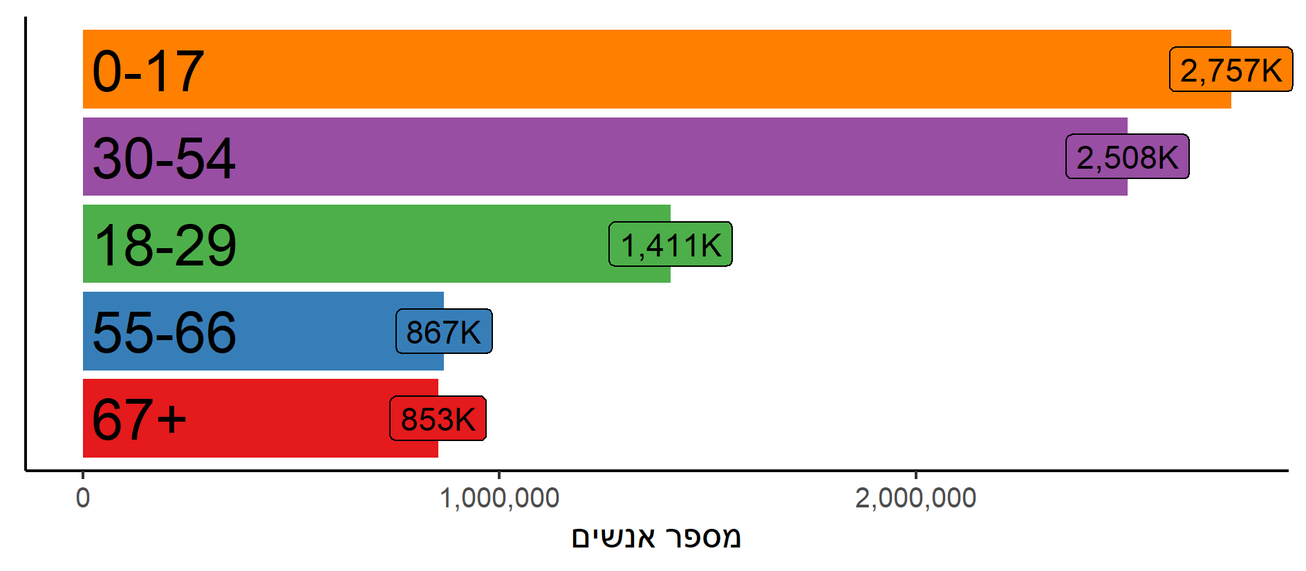
age_group2 = fct_collapse(as_factor(age_group),
"0-17" = as.character(c(1:4)),
"18-29" = as.character(c(5:6)),
"30-54" = as.character(c(7:11)),
"55-66" = as.character(c(12:15)),
"67+" = as.character(c(16:20))),
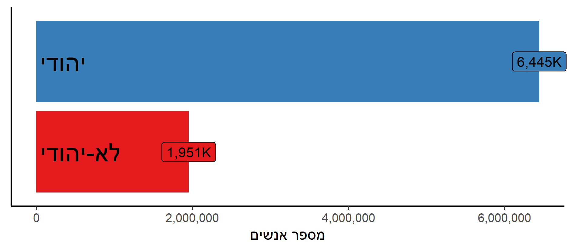
leom = if_else(nationality == 1, "יהודי",
"לא-יהודי"),
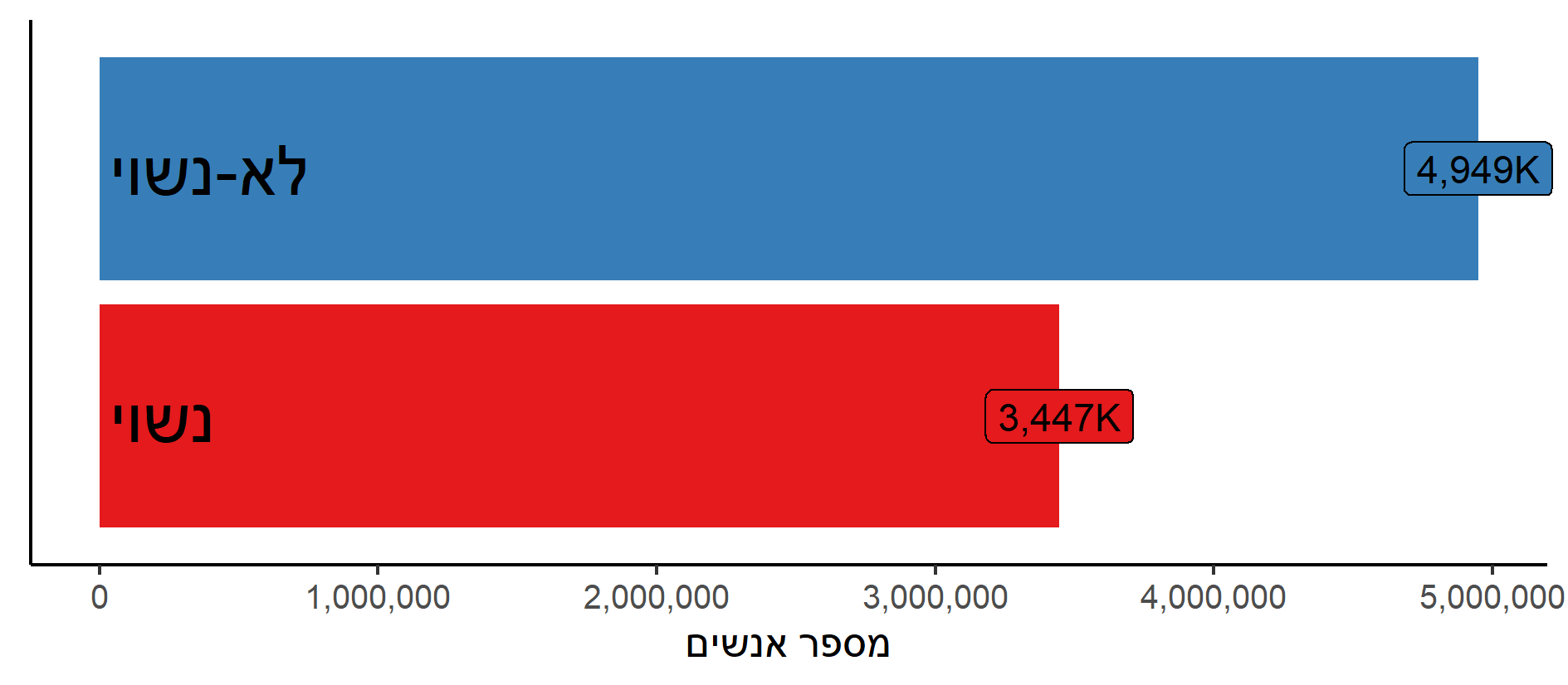
married = if_else(mazav_m == 1, "נשוי",
"לא-נשוי",
missing="לא-נשוי"),
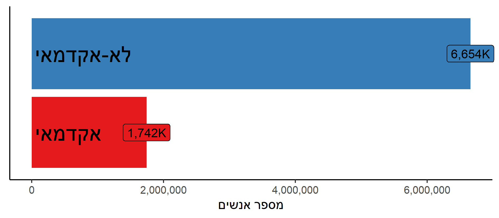
educ = if_else(between(sug_teuda, 5,7), "אקדמאי",
"לא-אקדמאי"),
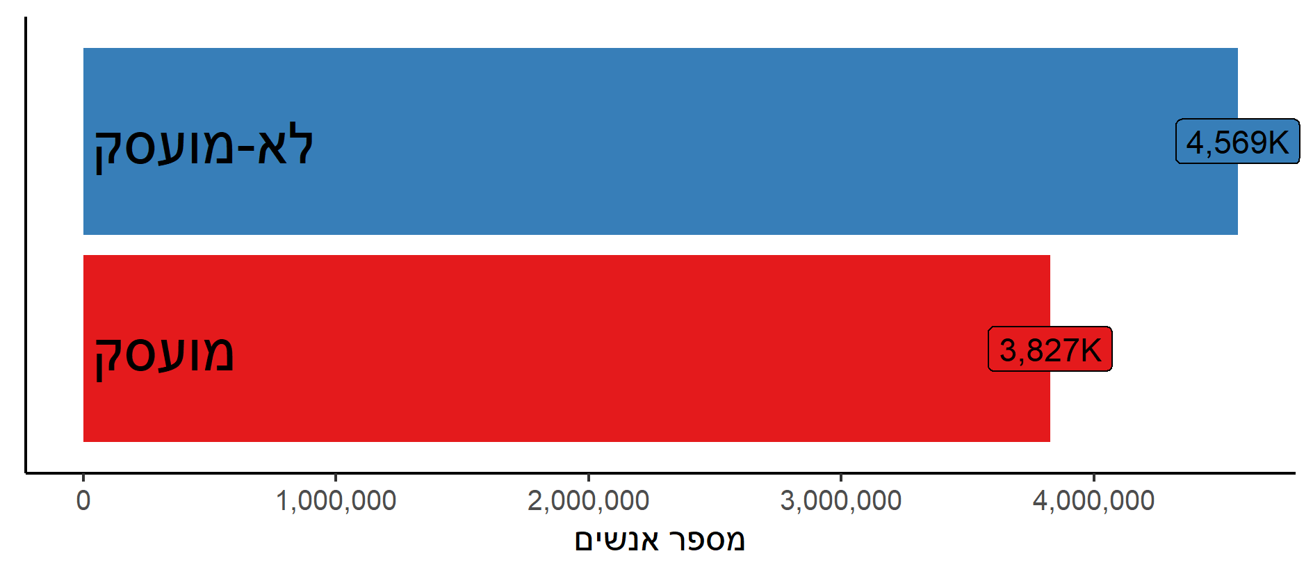
employed = if_else(avad == 1, "מועסק",
"לא-מועסק"),
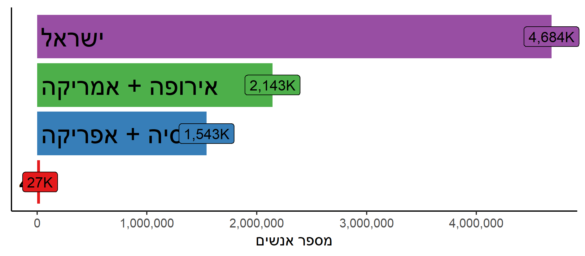
origin = if_else(yabeshet != 3, yabeshet, father_continent),
origin = fct_collapse(as_factor(origin),
"אירופה + אמריקה" = "1",
"אסיה + אפריקה" = "2",
"ישראל" = "3",
"לא-ידוע" = "4")
) %>%
left_join(read_csv("famexp_2017/H20171021datamb.csv") %>%
rename_all(tolower) %>%
select(misparmb, madadpereferia, decile, total_net, nefeshstandartit, ramatdatiyut, yshuv) %>%
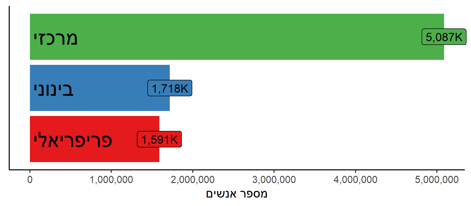
mutate(geo2 = fct_collapse(as_factor(madadpereferia),
"פריפריאלי" = c("1","2"),
"בינוני" = "3",
"מרכזי" = c("4","5")),
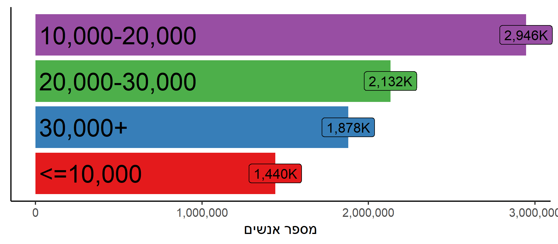
total_net_brackets = cut(total_net, breaks = c(-Inf, 10000, 20000, 30000, Inf), labels=FALSE),
total_net_brackets = fct_collapse(as_factor(total_net_brackets),
"<=10,000" = "1",
"10,000-20,000" = "2",
"20,000-30,000" = "3",
"30,000+" = "4"),
relig = ramatdatiyut
),
by = "misparmb"
) creating a new dataframe, with only the needed variables, and turning Arabs who marked themselves as “haredi” as “religious”:
data_reduced <- data %>%
select(misparmb, prat, sex, age_group2, leom, origin, relig, married, educ, employed, geo2, total_net_brackets, weight) %>%
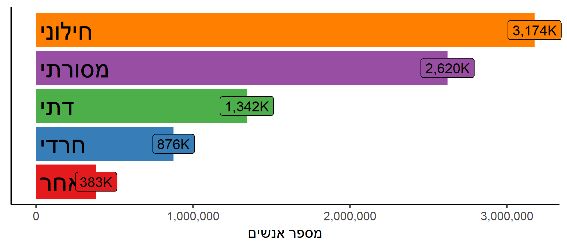
mutate(relig = if_else(leom == "לא-יהודי" & relig == 4,
3,
relig),
relig = fct_collapse(as_factor(relig),
"חילוני" = "1",
"מסורתי" = "2",
"דתי" = "3",
"חרדי" = "4",
"אחר" = as.character(5:6))
)Finding the mode in each:
groupbyvar_barplot <- function(DF, var) {
  g <- DF %>%
    group_by( !!sym(var) ) %>%
    tally(wt = weight) %>%
    ggplot(aes(x = reorder(!!sym(var),n) ,
               y = n,
               fill = reorder(!!sym(var),n),
               label = number(n, scale=10e-4,suffix="K",big.mark=","))) +
    geom_col() +
    geom_bar_text(aes(label = !!sym(var)), size = 20, reflow=TRUE, place = "left") +
    scale_fill_brewer(palette = "Set1") +
    geom_label() +
    coord_flip(clip = "off") +
    scale_y_continuous(labels = comma) +
    labs(y = "מספר אנשים",
         x = var ) +
    theme(legend.position = "none",
          axis.title.y=element_blank(),
        axis.text.y=element_blank(),
        axis.ticks.y=element_blank())

  ggsave(filename=paste(var,".png"), width=16, height=7, units = "cm")

}

map(data_reduced %>% select(-c(misparmb, prat, weight)) %>% names(),
    ~groupbyvar_barplot(DF = data_reduced, var = .x))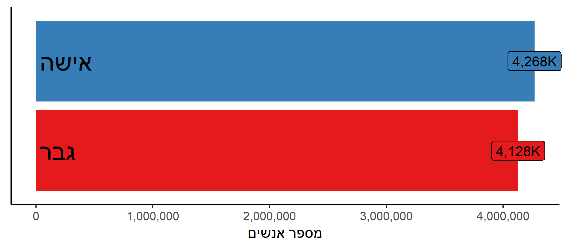
The Modal Israeli:
Pie chart plots:
All :
g1 <- data_reduced %>%
  group_by(sex, age_group2, leom, relig, origin, married, educ, employed, geo2, total_net_brackets) %>%
  tally(wt = weight) %>%
  mutate(group = paste(sex, age_group2, leom, relig, origin, married, educ, employed, geo2, total_net_brackets)) %>%
  ungroup() %>%
  select(group, n, sex) %>%
  arrange(desc(n)) %>%
  mutate(group = reorder(group, -n)) %>%
  head(n=5) %>%
  ggplot(aes(x="",y=n,fill=group,label = comma(n))) +
  geom_bar(stat="identity", width=1) +
  coord_polar("y", start = 0) +
  geom_text(position = position_stack(vjust = 0.5)) +
  theme_void() +
  theme(legend.position = "right",
        legend.text = element_text(size = 5)) +
  guides(fill = guide_legend(nrow=5, byrow=TRUE, title="", label.position = "left"))
Adults only:
g2 <- data_reduced %>%
  filter(age_group2 != "0-17") %>%
  group_by(sex, age_group2, leom, relig, origin, married, educ, employed, geo2, total_net_brackets) %>%
  tally(wt = weight) %>%
  mutate(group = paste(sex, age_group2, leom, relig, origin, married, educ, employed, geo2, total_net_brackets)) %>%
  ungroup() %>%
  select(group, n, sex) %>%
  arrange(desc(n)) %>%
  mutate(group = reorder(group, -n)) %>%
  head(n=5) %>%
  ggplot(aes(x="",y=n,fill=group,label = comma(n))) +
  geom_bar(stat="identity", width=1) +
  coord_polar("y", start = 0) +
  geom_text(position = position_stack(vjust = 0.5)) +
  theme_void() +
  theme(legend.position = "right",
        legend.text = element_text(size = 5)) +
  guides(fill = guide_legend(nrow=5, byrow=TRUE, title="", label.position = "left", ))
create manual legend labels, use slightly less ugly color palette and output plots to file:
biggest_groups1 <- c("גברים בני 0-17 יהודים חילונים ממוצא ישראלי לא-נשואים לא-אקדמאים לא-מועסקים צורת מגורים מרכז והכנסה של 30,000 שקלים ומעלה למשק בית",
"נשים בנות 0-17 יהודיות חילוניות ממוצא ישראלי לא-נשואות לא-אקדמאיות לא-מועסקות צורת מגורים מרכז והכנסה של 30,000 שקלים ומעלה למשק בית",
"גברים בני 0-17 יהודים חרדים ממוצא ישראלי לא-נשואים לא-אקדמאים לא-מועסקים צורת מגורים מרכז והכנסה בין 10,000 ל-20,000 שקלים למשק בית",
"נשים בנות 0-17 יהודיות חרדיות ממוצא ישראלי לא-נשואות לא-אקדמאיות לא-מועסקות צורת מגורים מרכז והכנסה בין 10,000 ל-20,000 שקלים ומעלה למשק בית",
"גברים בני 0-17 יהודים חילונים ממוצא ישראלי לא-נשואים לא-אקדמאים לא-מועסקים צורת מגורים מרכז והכנסה בין 20,000 ל-30,000 שקלים ומעלה למשק בית")

biggest_groups2 <- c("נשים בנות 30-54 יהודיות חילוניות ממוצא אירופאי או אמריקאי נשואות אקדמאיות מועסקות צורת מגורים מרכז והכנסה של 30,000 שקלים ומעלה למשק בית",
"גברים בני 30-54 יהודים חילונים ממוצא אירופאי או אמריקאי נשואים אקדמאים מועסקים צורת מגורים מרכז והכנסה של 30,000 שקלים ומעלה למשק בית",
"נשים בנות 30-54 יהודיות חילוניות ממוצא ישראלי נשואות אקדמאיות מועסקות צורת מגורים מרכז והכנסה של 30,000 שקלים ומעלה למשק בית",
"גברים בני 30-54 יהודים חילונים ממוצא ישראלי נשואים אקדמאים מועסקים צורת מגורים מרכז והכנסה של 30,000 שקלים ומעלה למשק בית",
"גברים בני 18-29 יהודים חילונים ממוצא ישראלי לא-נשואים לא-אקדמאים מועסקים צורת מגורים מרכז והכנסה של 30,000 שקלים ומעלה למשק בית")

g1 + scale_fill_brewer(labels = str_wrap(biggest_groups1, width=50), palette="Set1")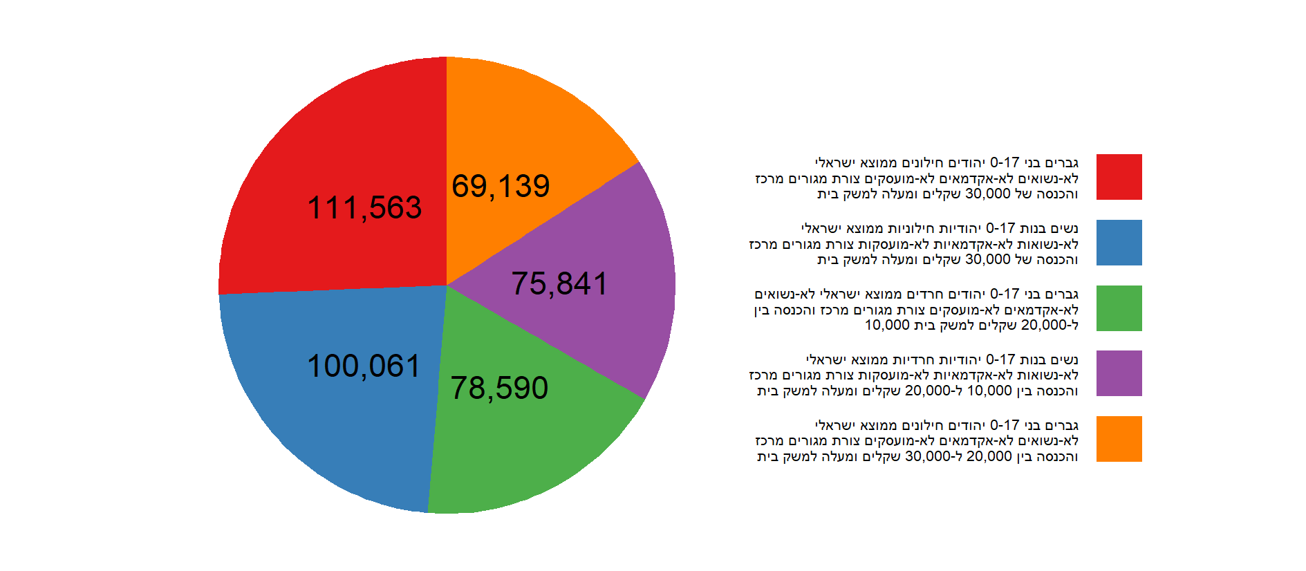
ggsave(filename="most_common_all_pie.png", width=16, height=7, units = "cm")

g2 + scale_fill_brewer(labels = str_wrap(biggest_groups2, width=50), palette = "Set1")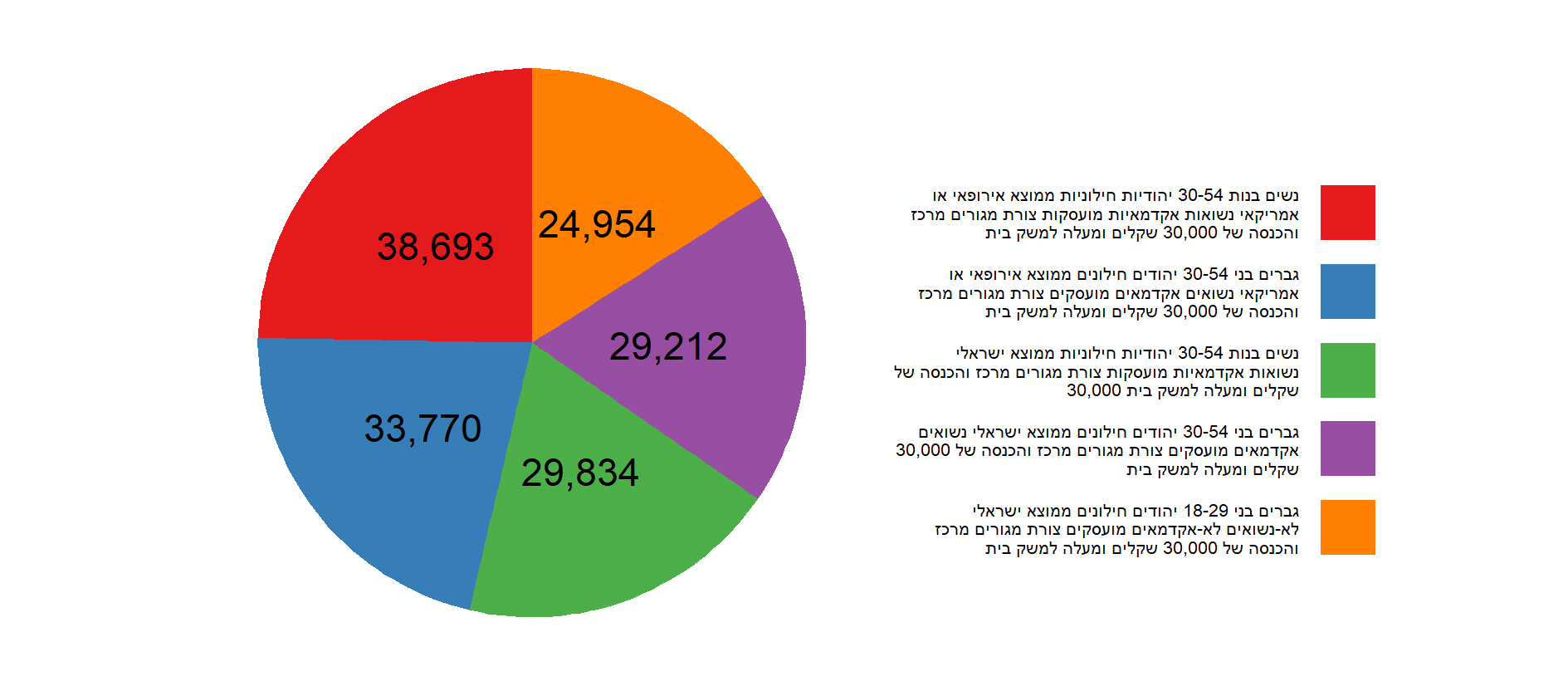
ggsave(filename="most_common_adults.png", width=16, height=7, units = "cm")